
Overview
When using Shoresim to compare scenarios, the most common mistake is running “different” simulations and treating the results as comparable.
A valid scenario comparison requires a controlled experiment:
-
only one thing changes between scenarios (the independent variable)
-
everything else stays fixed
This article explains the rules for valid comparisons, how to choose a defensible number of runs, and how to compare scenarios correctly.
1) Core Rule: Valid Comparisons Require Controlled Experiments
When comparing scenarios, all scenarios must have:
-
The same simulation duration
-
The same number of runs
-
The same model structure and complexity
-
Only one changed input (the independent variable)
If duration, run count, or complexity differ, observed KPI differences may be caused by:
-
Sampling variability (different run counts)
-
Time-horizon effects (different durations)
-
Structural effects (different model complexity)
These are confounding factors, meaning you can no longer attribute differences to the change you intended to test.
Key Terminology
-
Independent variable: the input you intentionally change between scenarios
-
Dependent variables: the KPIs you observe (availability, cost, downtime, etc.)
-
Confounders: unintended differences (duration, run count, complexity)
2) Shoresim Runs Are Independent
Shoresim produces independent random numbers across runs, meaning:
-
each run is statistically independent
-
scenario comparisons should use independent-sample statistical methods
-
paired-run methods do not apply
This is important when selecting statistical tests and interpreting confidence intervals.
3) How to Choose the Number of Runs (Sequential Precision Method)
The recommended approach is a standard sequential precision method, where you add runs until you reach a confidence target.
This avoids:
-
under-running (results too noisy to trust)
-
over-running (wasted sim minutes)
3.1 Define Acceptable Precision
Choose:
-
a confidence level (typically 95%)
-
a relative precision target γ (example: 3%)
Interpretation:
“The mean KPI value must be estimated with a confidence interval half-width less than γ of the mean.”
3.2 Confidence Interval Half-Width
After n runs, for KPI X:
-
sample mean: X̄
-
sample standard deviation: s
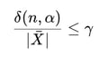
The confidence interval half-width is:
![]()
Stopping rule (relative half-width):
If the criterion is not satisfied:
-
add more runs
-
recompute
-
stop once satisfied
3.3 Practical Sequential Workflow
A common and effective workflow is:
-
Run an initial batch (commonly 10 runs)
-
Compute mean, standard deviation, and CI half-width
-
Check the relative half-width criterion
-
Add runs in batches (e.g., +5 runs)
-
Stop when the criterion is satisfied
4) Worked Example (Availability KPI)
Goal
-
KPI: availability
-
Confidence: 95%
-
Target: relative half-width ≤ 3%
After 10 Runs
Assume:
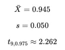
Half-width:
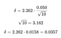
Relative half-width:
![]()
This does not meet the 3% target.
Estimating Required Runs
Since confidence interval half-width scales approximately with ![]() :
:
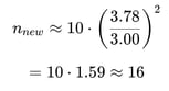
So you would increase to ~16 runs, recompute, and stop once the criterion is met.
5) Comparing Scenarios Correctly (Independent Two-Sample Method)
Because Shoresim runs are independent, Scenario A vs Scenario B comparisons should be done using:
-
the same simulation duration
-
the same number of runs
Then compute:
-
mean and variance for each scenario
-
a two-sample t confidence interval for the difference in means
What Not To Do
Do not compare:
-
Scenario A with 10 runs
-
Scenario B with 25 runs
Even if the numbers “look stable,” this is not a controlled experiment and can produce misleading conclusions.
6) Multiple Comparisons and Bonferroni Correction
When evaluating many KPIs, false positives become more likely.
A standard conservative correction is the Bonferroni correction:
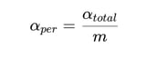
Example:
-
8 KPIs
-
overall α = 0.05
![]()
Effect of Bonferroni
-
wider confidence intervals
-
more conservative conclusions
-
more runs may be required
Recommendation:
Use Bonferroni for delivery-level reporting, not during early experimentation.
7) Further Reading
For a standard reference on simulation output analysis and experiment design:
-
Law, A. M. (2007), Simulation Modeling and Analysis
Covers confidence intervals, sequential stopping rules, two-sample comparisons, and multiple-comparison procedures (including Bonferroni).